If you are building a RAG application and already run Postgres, adding a second database just for embeddings often creates more pain than it solves. Using pgvector in Postgres lets you store embeddings, run similarity search, and keep your existing transactional data in one place. This tutorial walks through installing the extension, choosing the right index, writing efficient queries, and tuning it for production workloads.
The post is aimed at backend engineers who are comfortable with SQL and want a pragmatic path to vector search without spinning up Pinecone, Qdrant, or Weaviate. By the end, you will have a working schema, an index that fits your data shape, and a clear mental model of when pgvector is the right call.
What Is pgvector?
pgvector is an open-source Postgres extension that adds a vector data type plus exact and approximate nearest neighbor search. It supports cosine distance, L2 (Euclidean) distance, and inner product, and ships two index types built specifically for high-dimensional embeddings. Because it lives inside Postgres, you get joins, transactions, and ACID guarantees on your vector data for free.
The extension was created by Andrew Kane and is now maintained as an active open-source project with releases roughly every quarter. Major cloud providers offer it as a managed option: AWS RDS and Aurora, Google Cloud SQL, Azure Database for PostgreSQL, Supabase, and Neon all support pgvector without custom builds.
For most RAG workloads, pgvector handles the same retrieval patterns you would expect from a dedicated vector database. You insert an embedding alongside your row, build an index, and query with a distance operator. The difference is that the embedding sits next to your users, documents, or chunks table, so filtering by tenant, date, or category is just a regular WHERE clause.
Why pgvector Instead of a Dedicated Vector DB?
The honest answer is: usually because you already run Postgres, and a second database doubles your operational surface. Every extra piece of infrastructure means new backups, new monitoring, new failure modes, and one more thing to keep in sync. For teams under fifty engineers, that cost is real.
There are also concrete data-modeling wins. RAG pipelines almost always need metadata filters — tenant ID, document permissions, recency, source. In a dedicated vector store, those filters either run on a payload field with limited indexing, or force you to round-trip back to Postgres anyway. With pgvector, you write one query with a JOIN and a WHERE against indexed columns.
Here is how pgvector compares to the dedicated options on the dimensions that usually matter:
| Feature | pgvector | Pinecone | Qdrant | Weaviate |
|---|---|---|---|---|
| Hosting model | Self-host or managed Postgres | Managed only | Self-host or cloud | Self-host or cloud |
| Metadata filters | Native SQL with indexes | Payload filters | Payload filters | GraphQL filters |
| Transactions | Full ACID | None | None | None |
| Joins with relational data | Yes | No | No | No |
| Index types | HNSW, IVFFlat | HNSW (managed) | HNSW | HNSW |
| Hybrid search | Via tsvector or pg_trgm | Sparse-dense | Built-in | Built-in |
| Operational cost | Same as Postgres | Separate service | Separate service | Separate service |
The trade-off is throughput at very large scale. Once you are past roughly 50–100 million vectors and need sub-50ms p99 latency, a purpose-built engine starts to pull ahead on raw query speed and memory efficiency. For the 90% of teams who are below that scale, pgvector is usually the right starting point. If you want a deeper comparison across engines, see our guide on vector databases compared.
Installing pgvector
On a self-hosted Postgres, install the extension package and enable it inside the database:
-- Run as superuser inside your database
CREATE EXTENSION IF NOT EXISTS vector;

-- Verify it loaded
SELECT extname, extversion FROM pg_extension WHERE extname = 'vector';
On AWS RDS or Aurora PostgreSQL, the extension is available on engine versions 15.2 and later. You enable it the same way once you are connected. On Supabase, it is on by default for new projects, and the dashboard exposes it under Database → Extensions.
If you are running Postgres in Docker for local development, the official pgvector/pgvector:pg16 image saves you a build step:
docker run -d --name pg-rag \
  -e POSTGRES_PASSWORD=local \
  -p 5432:5432 \
  pgvector/pgvector:pg16
Once the container is up, the extension is already compiled and just needs CREATE EXTENSION vector inside whichever database you intend to use.
Storing Embeddings: Schema Design
The core decision is what dimension your vectors will be. OpenAI’s text-embedding-3-small produces 1536 dimensions, text-embedding-3-large produces 3072, and Cohere and Voyage models often use 1024. Pick the model first, then declare the column to match:
CREATE TABLE document_chunks (
  id          BIGSERIAL PRIMARY KEY,
  document_id BIGINT NOT NULL REFERENCES documents(id) ON DELETE CASCADE,
  chunk_index INT NOT NULL,
  content     TEXT NOT NULL,
  embedding   VECTOR(1536) NOT NULL,
  metadata    JSONB DEFAULT '{}'::jsonb,
  tenant_id   BIGINT NOT NULL,
  created_at  TIMESTAMPTZ NOT NULL DEFAULT now()
);

CREATE INDEX ON document_chunks (tenant_id);
CREATE INDEX ON document_chunks USING gin (metadata);
A few notes on this schema. The document_id foreign key with ON DELETE CASCADE means deleting a document automatically removes its chunks — useful when permissions change or content is retracted. The tenant_id column gets its own index so filtered searches are fast. The metadata JSONB column is the escape hatch for fields you have not yet promoted to first-class columns: page numbers, section headings, original URLs.
Inserting a row from Python using psycopg and the OpenAI SDK looks like this:
import os
import psycopg
from openai import OpenAI

client = OpenAI()
conn = psycopg.connect(os.environ["DATABASE_URL"])

def embed_and_store(document_id: int, chunk_index: int, text: str, tenant_id: int):
    response = client.embeddings.create(
        model="text-embedding-3-small",
        input=text,
    )
    embedding = response.data[0].embedding  # list[float] of length 1536

    with conn.cursor() as cur:
        cur.execute(
            """
            INSERT INTO document_chunks
              (document_id, chunk_index, content, embedding, tenant_id)
            VALUES (%s, %s, %s, %s, %s)
            """,
            (document_id, chunk_index, text, embedding, tenant_id),
        )
    conn.commit()
psycopg 3 will adapt a Python list of floats directly to pgvector’s text format. If you are on psycopg2, install the pgvector Python package and register its adapter once at startup.
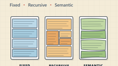
For the chunking step before embedding, the strategy you pick affects retrieval quality more than the database choice does. Our RAG chunking strategies guide covers the trade-offs between fixed-size, recursive, and semantic chunking.
HNSW vs IVFFlat: Choosing the Right Index
pgvector offers two approximate nearest neighbor indexes. Picking the wrong one is the single biggest performance mistake teams make on their first deploy.
HNSW (Hierarchical Navigable Small World) is a graph-based index that delivers better recall and lower query latency at the cost of slower builds and higher memory use. It is the right default for most workloads.
IVFFlat (Inverted File with Flat compression) partitions vectors into clusters and only searches the nearest clusters at query time. Builds are faster and memory use is lower, but recall and latency are worse than HNSW. Use it when you need to rebuild indexes frequently or memory is tight.
| Property | HNSW | IVFFlat |
|---|---|---|
| Build time | Slow (minutes to hours) | Fast (seconds to minutes) |
| Query latency | Lower | Higher |
| Recall at default settings | Higher | Lower |
| Memory footprint | Higher | Lower |
| Tunable parameters | m, ef_construction, ef_search | lists, probes |
| Updates without rebuild | Supported | Supported but recall degrades |
Create an HNSW index with cosine distance, which is what you want for OpenAI, Cohere, and most modern text embedding models:
CREATE INDEX ON document_chunks
USING hnsw (embedding vector_cosine_ops)
WITH (m = 16, ef_construction = 64);
The m parameter controls how many connections each node has in the graph; higher values improve recall but use more memory. The ef_construction parameter is how thoroughly the index is built; higher values produce a better graph but make the build slower. Defaults of 16 and 64 work well for most workloads up to a few million vectors.
If you genuinely need IVFFlat — for example, you are loading 50 million vectors and the HNSW build is too slow — pick the list count as roughly the square root of your row count:
CREATE INDEX ON document_chunks
USING ivfflat (embedding vector_cosine_ops)
WITH (lists = 1000);
For broader context on Postgres indexing, our database indexing strategies post covers when each index type pays for itself.
Querying: Cosine, L2, and Inner Product
pgvector exposes three distance operators. Use the one that matches how your embedding model was trained.
<=>— cosine distance (1 minus cosine similarity)<->— Euclidean (L2) distance<#>— negative inner product
For OpenAI, Cohere, Voyage, and most sentence-transformer models, cosine is the correct choice. A basic similarity query looks like this:
SELECT id, content, 1 - (embedding <=> $1) AS similarity
FROM document_chunks
WHERE tenant_id = $2
ORDER BY embedding <=> $1
LIMIT 10;
Notice the WHERE tenant_id = $2 filter. With a regular B-tree index on tenant_id, Postgres can scope the vector search to one tenant’s data efficiently. This is the kind of join-and-filter pattern that is awkward in dedicated vector stores.
To get the HNSW search to actually use the index, you have to keep the ORDER BY expression identical to what the index was built on. Mixing distance operators inside the same query is a common foot-gun:
-- BAD: this won't use the cosine HNSW index
SELECT * FROM document_chunks ORDER BY embedding <-> $1 LIMIT 10;

-- GOOD: matches the index ops class
SELECT * FROM document_chunks ORDER BY embedding <=> $1 LIMIT 10;
For HNSW, the runtime knob is ef_search. Higher values trade latency for recall:
SET LOCAL hnsw.ef_search = 100;  -- default is 40
SELECT id, content FROM document_chunks
ORDER BY embedding <=> $1
LIMIT 10;
Run this inside a transaction so the setting only affects that one query. For IVFFlat, the equivalent is ivfflat.probes.
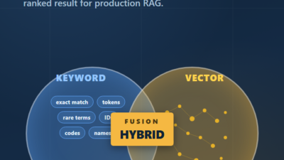
If your retrieval quality is poor at this stage, the embedding model is usually the culprit, not pgvector. Beyond that, consider combining vector search with keyword search — our hybrid search guide walks through fusing BM25 and vector scores.
Real-World Scenario: A Multi-Tenant Knowledge Base
Consider a B2B SaaS team building an internal knowledge search feature. They serve a few hundred customer organizations, each with their own document corpus ranging from a hundred to tens of thousands of pages. They already run Postgres on AWS RDS for the rest of the product.
In this kind of setup, adding Pinecone usually means introducing a separate tenant abstraction in the vector store, paying per-namespace overhead, and writing a sync job to keep document metadata aligned across two systems. With pgvector, the same workload lives in one database. A search query joins document_chunks against documents and tenants, filters by the requesting user’s organization, and returns the top-k results. Permissions, soft-deletes, and audit logs all live where they already do.
The practical limits worth knowing: with HNSW on RDS db.r6g.xlarge (4 vCPU, 32GB RAM), teams in this profile typically see p95 query latency under 50ms for top-10 retrieval against a few million chunks, as long as the index fits in shared_buffers. Once the working set spills to disk, latency climbs sharply, which is the signal to either upsize the instance or move to a dedicated engine.
Tuning pgvector for Production
A handful of settings make a disproportionate difference. Set maintenance_work_mem high enough that HNSW builds happen in memory — at least 2GB for indexes over a million rows. Increase shared_buffers to roughly 25% of available RAM so the index pages stay hot. For background writes, bump max_parallel_maintenance_workers so index builds use more cores.
-- Session-level tuning for a one-off index build
SET maintenance_work_mem = '4GB';
SET max_parallel_maintenance_workers = 4;
CREATE INDEX CONCURRENTLY ON document_chunks
USING hnsw (embedding vector_cosine_ops);
CREATE INDEX CONCURRENTLY is important on a live table — it avoids the long write lock that a plain CREATE INDEX takes. The trade-off is that the build is slower and uses more I/O overall.
On the application side, pool your connections. A vector query that hits an HNSW index is CPU-bound during the graph traversal; without pooling, connection overhead dominates at high QPS. The standard tools apply here — our database connection pooling guide covers PgBouncer and HikariCP setups.
Lastly, treat embedding writes as bulk-friendly. Use COPY or batched INSERT statements with 500–5000 rows per batch when you are backfilling. Embedding generation is the bottleneck at that scale, not Postgres, so parallelize the API calls and feed results in batches.
For the deeper Postgres tuning fundamentals — work_mem, autovacuum, query planning — see our PostgreSQL performance tuning post.
When to Use pgvector in Postgres
- You already run Postgres and want one less system to operate
- You need transactional consistency between embeddings and relational data
- Your retrieval queries combine vector similarity with metadata filters or joins
- You have under roughly 50 million vectors and p95 latency targets above 50ms
- Your team is small and operational simplicity outweighs squeezing the last 10ms
When NOT to Use pgvector in Postgres
- You need sub-10ms p99 latency at hundreds of millions of vectors
- Your team has dedicated infrastructure engineers and can absorb a second data store
- You need built-in features like sparse-dense hybrid search or learned reranking that pgvector does not ship natively
- You are running embeddings at a scale where memory cost in Postgres becomes prohibitive
- Your Postgres instance is already strained on CPU or I/O for transactional workloads
Common Mistakes with pgvector
- Building HNSW indexes without raising
maintenance_work_mem, which makes builds take 10x longer than they should - Forgetting to filter by tenant or permission before vector search, which both leaks data and slows queries
- Using
<->(L2) in queries when the index was built withvector_cosine_ops, silently bypassing the index - Storing embeddings as JSON or text columns instead of the native
vectortype, breaking the ability to index - Re-embedding on every read instead of caching, which puts the OpenAI API on your hot path
- Skipping
CREATE INDEX CONCURRENTLYon a live table and blocking writes during a long index build
Wrapping Up
pgvector in Postgres is the right default for most teams starting with RAG. You get vector similarity search, full SQL filtering, and ACID transactions in the database you already run. The main upgrade triggers are query latency at very high scale and feature gaps like native hybrid search, neither of which apply to most production apps.
If you are coming from a first prototype, your next step is to pick chunking and embedding choices carefully — those decide retrieval quality far more than the index does. Start with our RAG from scratch walkthrough if you need the end-to-end pipeline, and then layer in hybrid search once basic retrieval is working.
3 Comments