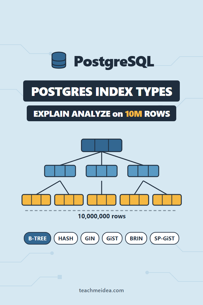
Most advice about Postgres index types stops at a sentence per type: B-tree for ordering, GIN for arrays, BRIN for time series. That is correct and nearly useless, because it never tells you what each one costs. This post builds one 10-million-row table, puts twenty-two indexes on it one at a time, and reports the build time, the size on disk and the EXPLAIN ANALYZE execution time for every single one.
This is for developers who own a schema that has outgrown its first index and now have to justify the next one. Specifically, it answers three questions the documentation leaves open: how much disk does each index type actually consume, how much faster does it make a realistic query, and when does the planner quietly refuse to use it at all. Three of the results below contradict advice you have probably been given.
How These Postgres Index Types Were Measured
Every number came from a PostgreSQL 18.4 server built from the official EDB Windows binaries, running on a throwaway cluster with stock initdb settings. Nothing was tuned, because the point is to show what the defaults do to a table this size.
Measured 2026-09-15
Windows 11 Pro 25H2 (build 26200), AMD Ryzen 5 8600G (6C/12T), 15.2 GB RAM, Kingston SNV2S1000G NVMe SSD
PostgreSQL 18.4 on x86_64-windows, compiled by msvc-19.44.35226
Database encoding UTF8, ICU collation en-US, default_text_search_config pg_catalog.english
shared_buffers 128MB, work_mem 4MB, maintenance_work_mem 64MB, effective_cache_size 4GB
random_page_cost 4, seq_page_cost 1, jit on
max_parallel_workers_per_gather 2, max_parallel_maintenance_workers 2
Query timings vary between runs, so each query ran six times: one warm-up that is discarded, then five measured runs. The reported figure is the median of those five. The harness parses the Execution Time field out of EXPLAIN (ANALYZE, BUFFERS, FORMAT JSON), which means the numbers exclude network round trips and client-side result handling.
Index sizes and build times were captured differently. Each index was created alone, timed with clock_timestamp(), measured with pg_relation_size(), then dropped before the next variant was created. Consequently no result below benefits from a second index that happened to be sitting there. Sizes do not vary between runs, so no repeat count applies to them.
Here is the timing function, which you can paste into any database to reproduce the method:
-- Runs a query six times, discards the first, records the median of the rest.
-- EXPLAIN ANALYZE is used rather than \timing so the number excludes the round trip.
CREATE OR REPLACE FUNCTION bench(p_shape text, p_variant text, p_query text, p_runs int DEFAULT 5)
RETURNS void AS $$
DECLARE
  plan json;
  arr  numeric[] := '{}';
BEGIN
  EXECUTE 'EXPLAIN (ANALYZE, BUFFERS, FORMAT JSON) ' || p_query INTO plan;  -- warm-up
  FOR i IN 1..p_runs LOOP
    EXECUTE 'EXPLAIN (ANALYZE, BUFFERS, FORMAT JSON) ' || p_query INTO plan;
    arr := arr || round((plan->0->>'Execution Time')::numeric, 3);
  END LOOP;
  INSERT INTO qbench (shape, variant, median_ms, runs_ms)
  SELECT p_shape, p_variant,
         (SELECT percentile_cont(0.5) WITHIN GROUP (ORDER BY x) FROM unnest(arr) x), arr;
END $$ LANGUAGE plpgsql;
The Table Every Number Came From
The table models an events log, because that shape puts every index type under load: a high-cardinality foreign key, a low-cardinality status, a monotonic timestamp, an array, a JSONB document and a text field.
CREATE TABLE events (
  id           bigint      NOT NULL,
  user_id      integer     NOT NULL,
  status       text        NOT NULL,
  country      char(2)     NOT NULL,
  amount_cents integer     NOT NULL,
  created_at   timestamptz NOT NULL,
  tags         text[]      NOT NULL,
  payload      jsonb       NOT NULL,
  title        text        NOT NULL
);
Rows are generated deterministically from generate_series rather than from random(), so the same script produces a byte-identical table on any machine. After VACUUM ANALYZE, the heap occupies 1,995 MB across 10,000,000 rows.
The distributions matter more than the schema, because selectivity drives every result below:
| Column | Distribution |
|---|---|
user_id | 200,000 distinct values, 50 rows each |
status | paid 6,000,000 (60%), shipped 2,300,000 (23%), pending 1,000,000 (10%), refunded 500,000 (5%), cancelled 200,000 (2%) |
created_at | strictly increasing, 2 seconds apart, spanning 231 days |
tags | 200 distinct three-element sets, 50,000 rows each |
payload | {"plan": ..., "region": ..., "v": ...}, plan has 4 values |
title | four words drawn from a 64-word vocabulary |
Postgres Index Types: Size and Build Time on 10 Million Rows
This is the table that is missing from most discussions. Every index below covers the same 10 million rows, and the spread between the smallest and the largest is a factor of 24,000.
| Index | Type | Build time | Size |
|---|---|---|---|
created_at | BRIN (default) | 0.5 s | 80 kB |
created_at | BRIN (pages_per_range=32) | 0.5 s | 280 kB |
created_at WHERE status='cancelled' | B-tree partial | 0.4 s | 4.3 MB |
payload jsonb_path_ops | GIN | 2.5 s | 43 MB |
to_tsvector('english', title) | GIN | 14.4 s | 53 MB |
tags | GIN | 5.1 s | 54 MB |
status | B-tree | 3.7 s | 66 MB |
(payload->>'plan'), (payload->>'v') | B-tree expression | 8.5 s | 66 MB |
user_id | B-tree | 2.5 s | 68 MB |
title | B-tree | 4.9 s | 68 MB |
title text_pattern_ops | B-tree | 4.3 s | 68 MB |
payload | GIN (jsonb_ops) | 5.9 s | 75 MB |
(user_id, amount_cents) | B-tree | 2.8 s | 90 MB |
created_at | B-tree | 2.5 s | 214 MB |
user_id INCLUDE (amount_cents) | B-tree covering | 3.2 s | 215 MB |
user_id | Hash | 9.8 s | 298 MB |
(created_at, status) | B-tree | 3.1 s | 306 MB |
(status, created_at) | B-tree | 6.9 s | 307 MB |
title | SP-GiST | 56.0 s | 307 MB |
title gin_trgm_ops | GIN trigram | 21.2 s | 333 MB |
to_tsvector('english', title) | GiST | 155.4 s | 695 MB |
title gist_trgm_ops | GiST trigram | 117.2 s | 1,890 MB |
Two rows deserve immediate attention. The GiST trigram index is 1,890 MB against a 1,995 MB table, so it very nearly doubles the storage for that one table. Meanwhile the BRIN index on created_at covers the same 10 million rows in 80 kB, which is 2,742 times smaller than the B-tree on the identical column.
That B-tree gap is not a typo either. btree(user_id) is 68 MB while btree(created_at) is 214 MB, even though both index one column. The reason is B-tree deduplication: user_id has only 200,000 distinct values repeated 50 times each, so Postgres stores one key with a posting list of row pointers. Every created_at value is unique, therefore nothing deduplicates.
What the Postgres Index Types Can Actually Do
Before the timings, the capability matrix decides most arguments on its own. Postgres index types differ in capability before they differ in speed, and these values were read out of the running server with pg_indexam_has_property() rather than copied from documentation:
| Access method | Ordered scans | UNIQUE | Multicolumn | INCLUDE |
|---|---|---|---|---|
| B-tree | Yes | Yes | Yes | Yes |
| Hash | No | No | No | No |
| GiST | No | No | Yes | Yes |
| SP-GiST | No | No | No | Yes |
| GIN | No | No | Yes | No |
| BRIN | No | No | Yes | No |
B-tree is the only type that can serve ORDER BY from the index, and the only one that can enforce a unique constraint. That single row explains why B-tree remains the default answer despite everything below.
B-tree vs Hash for Equality: A 26,000x Speedup
Start with the simplest case, an equality lookup returning 50 rows out of 10 million. Without an index, Postgres reads the whole table:
EXPLAIN (ANALYZE, BUFFERS)
SELECT id, created_at, amount_cents FROM events WHERE user_id = 12345;
 Gather  (cost=1000.00..308447.43 rows=51 width=20) (actual time=1.590..389.717 rows=50.00 loops=1)
   Workers Planned: 2
   Workers Launched: 2
   Buffers: shared hit=15722 read=239637
   ->  Parallel Seq Scan on events  (cost=0.00..307442.33 rows=21 width=20) (actual time=11.238..357.753 rows=16.67 loops=3)
         Filter: (user_id = 12345)
         Rows Removed by Filter: 3333317
         Buffers: shared hit=15722 read=239637
 Planning Time: 0.098 ms
 Execution Time: 389.755 ms
Add a B-tree and the same query touches 53 buffers instead of 255,359:
 Index Scan using r_btree_user on events  (cost=0.43..209.33 rows=51 width=20) (actual time=0.057..0.660 rows=50.00 loops=1)
   Index Cond: (user_id = 12345)
   Buffers: shared hit=1 read=52
 Execution Time: 0.678 ms
| Variant | Median | Size |
|---|---|---|
| No index | 320.490 ms | — |
| B-tree | 0.012 ms | 68 MB |
| Hash | 0.013 ms | 298 MB |
The B-tree is 26,700 times faster than the sequential scan here. Hash matches it to within a microsecond, which is a tie. However, the hash index costs 298 MB against the B-tree’s 68 MB and takes 9.8 seconds to build against 2.5. Since it also cannot do ranges, ordering, uniqueness or multiple columns, there is no case in this data where hash wins. That result is consistent across every equality test run.
Low-Cardinality Columns: When the Planner Ignores Your Index
Here is the first result that contradicts common advice. A B-tree on status exists, and the planner uses it only for the rarest value.
| Query | Rows matched | No index | With B-tree |
|---|---|---|---|
status = 'cancelled' | 200,000 (2%) | 451.811 ms | 366.209 ms |
status = 'refunded' | 500,000 (5%) | 458.625 ms | 330.237 ms |
status = 'paid' | 6,000,000 (60%) | 771.360 ms | 817.115 ms |
At 60% selectivity the index is not merely useless, it is slightly worse, because the planner still pays to consider it and then scans the table anyway. At 5% the plan shows Gather -> Seq Scan, meaning the index was built, stored and ignored. Only at 2% does a bitmap scan appear, and even then the gain is 19%.
Notably, the bitmap plan reveals why the payoff is so small:
 ->  Parallel Bitmap Heap Scan on events  (actual time=10.383..315.042 rows=66666.67 loops=3)
       Recheck Cond: (status = 'cancelled'::text)
       Rows Removed by Index Recheck: 1249715
       Heap Blocks: exact=18872 lossy=45441
Those lossy heap blocks are the story. With work_mem at the default 4 MB, the bitmap could not hold one bit per row, so Postgres degraded it to one bit per page and re-checked 1.25 million rows it did not need. Raising work_mem is the fix, which is covered more broadly in PostgreSQL performance tuning.
A partial index looked like the obvious answer and came out worse:
| Variant | Median | Size |
|---|---|---|
B-tree on status | 366.209 ms | 66 MB |
Partial index WHERE status='cancelled' | 853.933 ms | 4.3 MB |
The partial index is 15 times smaller, which is real and valuable. Nevertheless it was 2.3 times slower here, because the planner chose a single-threaded Index Scan over it rather than a parallel bitmap scan, and 200,000 individual heap lookups beat the bitmap only when the rows are physically clustered. Partial indexes earn their keep on write cost and disk, not automatically on read latency.
BRIN vs B-tree on a Timestamp: 80 kB Against 214 MB
created_at increases with physical row order, which is the exact condition BRIN is designed for. BRIN stores a min and max per block range instead of an entry per row.
| Query | No index | B-tree (214 MB) | BRIN (80 kB) |
|---|---|---|---|
| One day, 43,200 rows | 351.273 ms | 2.852 ms | 4.714 ms |
| 30 days, 1,296,000 rows | 377.813 ms | 57.932 ms | 98.820 ms |
ORDER BY created_at DESC LIMIT 100 | 407.926 ms | 0.030 ms | 405.402 ms |
For the one-day range, BRIN costs 65% more time and 0.04% of the space. Dropping pages_per_range to 32 made it larger (280 kB) and slower (5.954 ms), so the default of 128 was the better setting on this data.
The third row is where BRIN collapses. Because BRIN cannot return rows in order, ORDER BY ... LIMIT 100 falls back to sorting the whole table: 405 ms against the B-tree’s 0.030 ms, a 13,500x difference. Any endpoint that paginates by timestamp needs the B-tree, whatever the disk saving looks like. If your workload is genuinely append-only time series, time-series data in PostgreSQL with TimescaleDB covers the partitioning approach that pairs with BRIN.
GIN for Arrays and JSONB: Selectivity Decides Everything
GIN indexes invert a composite value into its elements. Among the Postgres index types they are the most sensitive to selectivity, because they help enormously or barely at all depending on how many rows survive the filter.
| Query | Rows matched | No index | GIN |
|---|---|---|---|
tags @> ARRAY['tag42'] | 150,000 (1.5%) | 446.597 ms | 353.106 ms |
tags @> ARRAY['tag31','tag97'] | 50,000 (0.5%) | 586.035 ms | 137.570 ms |
At 1.5% the GIN index returned a 21% improvement for 54 MB, which is a poor trade. At 0.5% it returned 4.3x. The pattern repeats on JSONB:
| Query | Rows matched | No index | GIN jsonb_ops | GIN jsonb_path_ops |
|---|---|---|---|---|
payload @> '{"plan":"enterprise","v":7}' | 100,000 (1%) | 465.697 ms | 363.452 ms | 274.439 ms |
payload @> '{"plan":"enterprise"}' | 2,500,000 (25%) | 468.581 ms | 482.590 ms | 487.027 ms |
The second row is an honest negative result: at 25% selectivity both GIN indexes were slower than having no index at all. The planner still reads 2.5 million heap rows, and the index scan is pure overhead on top.
Between the two operator classes, jsonb_path_ops won on both axes: 274 ms against 363 ms, and 43 MB against 75 MB. The trade is that it only supports the @> containment operator, whereas the default jsonb_ops also handles key-existence operators such as ?. More JSONB schema guidance lives in PostgreSQL JSONB best practices.
A B-tree expression index on the two extracted keys was the slowest option at 496.763 ms, because extracting payload->>'plan' still forces a heap visit per row.
Full-Text Search: GIN and GiST Tie on Speed, Not on Cost
Searching to_tsvector('english', title) without an index is the worst number in this entire post, because Postgres has to build a tsvector for all 10 million rows on every execution.
| Variant | Median | Build time | Size |
|---|---|---|---|
| No index | 7,698.974 ms | — | — |
| GIN | 3,264.379 ms | 14.4 s | 53 MB |
| GiST | 3,226.374 ms | 155.4 s | 695 MB |
GiST and GIN finished within 38 ms of each other, which is a tie at this scale. The cost side is not close at all: GiST took 10.8 times longer to build and 13.1 times more disk for the same answer. Consequently GIN is the correct default for full-text, which matches the official recommendation. For the wider build-versus-buy question, see full-text search in PostgreSQL vs Elasticsearch vs Algolia.
Both indexes cut the time by 58% rather than eliminating it, because 156,250 rows still had to be fetched from the heap and counted.
Trigram Indexes: Worthless at 1.6%, 158x at 0.01%
Substring search with LIKE '%...%' cannot use a normal B-tree, so pg_trgm exists to index three-character fragments. On the title column the result was close to nothing:
| Variant | Median | Size |
|---|---|---|
| No index | 443.993 ms | — |
| GIN trigram | 389.007 ms | 333 MB |
| GiST trigram | 401.469 ms | 1,890 MB |
Spending 1,890 MB to save 42 ms is indefensible. However, that conclusion is an artifact of the data rather than of trigram indexes, because title draws from a 64-word vocabulary and the pattern matched 156,250 rows. Real substring search runs against identifiers.
So a second table was built to test that properly: 2,000,000 rows of email addresses, 118 MB, high cardinality.
| Query | Rows matched | No index | GIN trigram | GiST trigram |
|---|---|---|---|---|
email LIKE '%7391@%' | 200 (0.01%) | 70.644 ms | 0.448 ms | 28.366 ms |
email LIKE '%391@%' | 2,000 (0.1%) | 72.154 ms | 1.145 ms | — |
On selective substrings the GIN trigram index is 158 times faster, and it beats GiST by 63x while costing 64 MB against 232 MB. The lesson generalises: a trigram index is worth its considerable size only when the pattern eliminates almost every row.
Prefix LIKE: The Collation Trap That Costs 16.6x
This is the second result that contradicts common advice, and it catches people constantly. Under any non-C collation, a plain B-tree cannot perform a prefix search, even though it looks like it should. The database here uses ICU en-US, which is what a modern production cluster looks like.
-- B-tree with default operator class: scans the entire index, filters afterwards
 ->  Parallel Index Only Scan using r_btree_title on events (actual time=51.618..163.878 rows=52083.33 loops=3)
       Filter: (title ~~ 'granite%'::text)
       Rows Removed by Filter: 3281250
 Execution Time: 198.043 ms
-- Same column, text_pattern_ops: a genuine range seek
 ->  Index Only Scan using r_btree_title_pat on events (actual time=0.061..10.246 rows=156250.00 loops=1)
       Index Cond: ((title ~>=~ 'granite'::text) AND (title ~<~ 'granitf'::text))
 Execution Time: 14.245 ms
| Variant | Median | Size |
|---|---|---|
| No index | 438.326 ms | — |
| B-tree, default operator class | 210.100 ms | 68 MB |
B-tree, text_pattern_ops | 12.636 ms | 68 MB |
| SP-GiST | 26.267 ms | 307 MB |
Both B-trees are exactly 68 MB. The only difference is the operator class, and it is worth 16.6x. SP-GiST handled the prefix correctly without the opclass, but it took 56 seconds to build and 4.5 times the disk, so text_pattern_ops wins outright.
Covering Indexes: The INCLUDE That Cost 125 MB More
An index-only scan avoids the heap entirely, provided every column the query needs lives in the index.
| Variant | Median | Size | Plan |
|---|---|---|---|
| No index | 450.306 ms | — | Seq Scan |
B-tree (user_id) | 5.046 ms | 68 MB | Bitmap Heap Scan |
B-tree (user_id) INCLUDE (amount_cents) | 0.948 ms | 215 MB | Index Only Scan |
B-tree (user_id, amount_cents) | 1.203 ms | 90 MB | Index Only Scan |
The INCLUDE index is the fastest at 0.948 ms, and it is also the most expensive by a wide margin. The plain two-column index reached 1.203 ms, which is 27% slower, while occupying 90 MB instead of 215 MB. That is 125 MB saved for a quarter-millisecond.
The size difference has the same cause as earlier: included columns are payload rather than key data, so they cannot be deduplicated, whereas (user_id, amount_cents) as a compound key can be. Unless you need INCLUDE to keep a unique constraint on the leading column alone, the ordinary multicolumn index is usually the better deal. Index-only scans also require a recently vacuumed table, since Heap Fetches: 0 depends on the visibility map being current.
Multicolumn Column Order: 12.3x From Swapping Two Words
Same two columns, same query, same row count. Only the order in the CREATE INDEX statement changes.
| Index | Median | Size |
|---|---|---|
(status, created_at) | 1.740 ms | 307 MB |
(created_at, status) | 21.325 ms | 306 MB |
| No index | 433.607 ms | — |
The query filters status = 'cancelled' and a one-month created_at range. With status first, the index seeks directly to the 25,920 matching entries and reads 133 buffers. With created_at first, it must scan every entry in the month-long range and filter, reading 5,077 buffers. The rule is the familiar one, now with a number attached: equality columns come before range columns, and getting it backwards costs 12.3x.
What Indexes Cost on Write
Read gains are only half the decision. Inserting 100,000 rows into a copy of the table, with and without five ordinary indexes:
-- No indexes
INSERT 0 100000
Time: 606.997 ms

-- With btree(user_id), btree(created_at), btree(status), gin(tags), gin(payload jsonb_path_ops)
INSERT 0 100000
Time: 1538.632 ms
Five indexes made the insert 2.5 times slower. Therefore an index that delivers a 19% read improvement, like the status B-tree at its best case of 2% selectivity, is losing money on any write-heavy table.
What These Numbers Change in a Real Schema
Consider a reporting table in a mid-sized SaaS product, somewhere in the tens of millions of rows, maintained by a small backend team. The usual pattern is that indexes accumulate one incident at a time: a slow dashboard adds one, a slow export adds another, and nobody removes any.
The measurements above suggest three concrete audits for that situation, each of which turns on picking between Postgres index types rather than adding another one. First, any index on a column whose common value covers more than about 5% of the table is probably never being chosen by the planner, and pg_stat_user_indexes.idx_scan will confirm it in seconds. Second, a created_at B-tree on an append-only table is a candidate for BRIN, but only if nothing paginates by that column, which is a question about the API rather than the database. Third, any INCLUDE added for an index-only scan deserves a comparison against the plain multicolumn form, because the compound key may be less than half the size.
The trade-off worth stating plainly is that none of this is free to change. Dropping an index is instant, but rebuilding it if you were wrong takes minutes on a table this size and locks writes unless you use CREATE INDEX CONCURRENTLY. The safer sequence is to measure with idx_scan first, drop during a low-traffic window, and keep the CREATE INDEX statement in the migration that removed it. That pattern fits the broader approach in database migrations in production.
When to Use Each Postgres Index Type
Default to B-tree when
- The column is used for equality, ranges, sorting or a unique constraint
- The query needs
ORDER BY ... LIMIT, which no other type can serve from the index - You want the smallest index on a low-cardinality column, where deduplication shrinks it dramatically
Switch to BRIN when
- Values correlate strongly with physical row order, typically an append-only timestamp
- The table is large enough that a 214 MB B-tree is a real cost
- Range scans are the access pattern and ordered output is never required
Pick GIN when
- The column is an array, a JSONB document or a tsvector
- Queries match less than roughly 1% of the table
- Build time and disk matter, because GIN beat GiST on both in every test here
Add text_pattern_ops when
- The database uses any collation other than C and queries do prefix
LIKE - The alternative would be a 307 MB SP-GiST index for the same capability
Reserve trigram indexes for
- Substring search on high-cardinality text such as emails, SKUs or usernames
- Patterns selective enough to eliminate 99% of rows or more
When NOT to Use Each Postgres Index Type
Skip a B-tree on status-style columns when
- The values you actually filter on cover more than about 5% of rows
- The table takes heavy writes, since five indexes cost 2.5x on insert here
Avoid BRIN when
- Rows arrive out of order, or the column is updated after insert
- Anything paginates or sorts by that column, which cost 405 ms against 0.030 ms
Rule out hash indexes when
- Any other access pattern than single-column equality is plausible
- Disk matters, because hash needed 298 MB to tie a 68 MB B-tree
Decline GiST for text when
- The workload is full-text or trigram search and GIN is available
- 695 MB and 155 seconds of build time buy nothing measurable over GIN’s 53 MB
Think twice about INCLUDE when
- A plain multicolumn index would answer the same query, at 90 MB against 215 MB
- The table is not vacuumed often enough for index-only scans to skip the heap
Common Mistakes with Postgres Index Types
- Indexing a boolean or a five-value status column and assuming the planner will use it. At 60% selectivity it was measurably slower than no index at all.
- Treating
EXPLAINas proof. OnlyEXPLAIN ANALYZEreports what happened; the cost estimates are the planner’s guess, andRows Removed by Index Recheckis invisible without it. - Leaving
work_memat 4 MB and then blaming the index when a bitmap scan goes lossy and re-checks 1.25 million rows. - Creating a plain B-tree for prefix
LIKEunder a non-C collation. It builds, it is used, and it is 16.6 times slower than the same index withtext_pattern_ops. - Putting the range column before the equality column in a multicolumn index, which cost 12.3x here for a one-word change.
- Adding
INCLUDEreflexively for index-only scans without comparing it to the compound key, which was 58% smaller in this test. - Measuring index benefit without measuring insert cost on the same table.
What This Benchmark Does Not Measure
These Postgres index types were compared on one synthetic table on one machine, and several limitations follow directly from that.
Most importantly, the data is deterministic rather than random, which makes it reproducible but also unusually regular. The tags column has only 200 distinct sets, so no array query below 0.5% selectivity was possible to construct. Likewise title draws from 64 words, which is why the trigram test needed a second table to say anything useful.
The server ran with stock initdb settings on a 15.2 GB machine, so shared_buffers was 128 MB against a 1,995 MB table. A production server with 32 GB of RAM and a tuned shared_buffers would show smaller gaps between indexed and unindexed queries, because more of the heap would be resident.
Nothing here measures index bloat over time, REINDEX cost, replication lag from WAL volume, or behaviour under concurrent writes. All timings are single-session. Index build times used maintenance_work_mem at its 64 MB default and two parallel maintenance workers; raising either changes those numbers substantially. Finally, this is Windows on an NVMe SSD, and the relative ordering of results should hold on Linux while the absolute milliseconds will not.
For foundational material on choosing what to index before choosing how, database indexing strategies is the companion to this post.
Conclusion
The measured answer on Postgres index types is that B-tree deserves its default status and the alternatives are specialists with narrow, well-defined wins. B-tree was fastest or tied in every category it can serve, and it is the only type that handles ordering and uniqueness. Hash tied it on the one thing hash can do while costing 4.4 times the disk, so it has no role here.
Three results are worth carrying away because they contradict standard advice. A partial index came out 2.3 times slower than the full B-tree it replaced, despite being 15 times smaller. GIN on a 25% JSONB match was slower than no index at all. And a plain B-tree under ICU collation was 16.6 times slower at prefix LIKE than the identical index with text_pattern_ops, at exactly the same 68 MB.
The practical recommendation is to stop choosing index types by column data type and start choosing by selectivity. Below roughly 1% matched rows, almost any appropriate index wins big. Above about 5%, most of them lose to a sequential scan, and you are paying 2.5x on writes for nothing.
The concrete next step takes about a minute. Run this against your own database, and every index it lists with a low scan count is a candidate for deletion:
SELECT relname AS table_name, indexrelname AS index_name,
       idx_scan, pg_size_pretty(pg_relation_size(indexrelid)) AS size
FROM pg_stat_user_indexes
ORDER BY idx_scan ASC, pg_relation_size(indexrelid) DESC
LIMIT 20;